Truncating Embeddings Works Without Matryoshka, Up to a Point
Truncating embeddings supposedly needs Matryoshka training. A 2026 study across 24 tasks found plain truncation holds until you cut 80%.
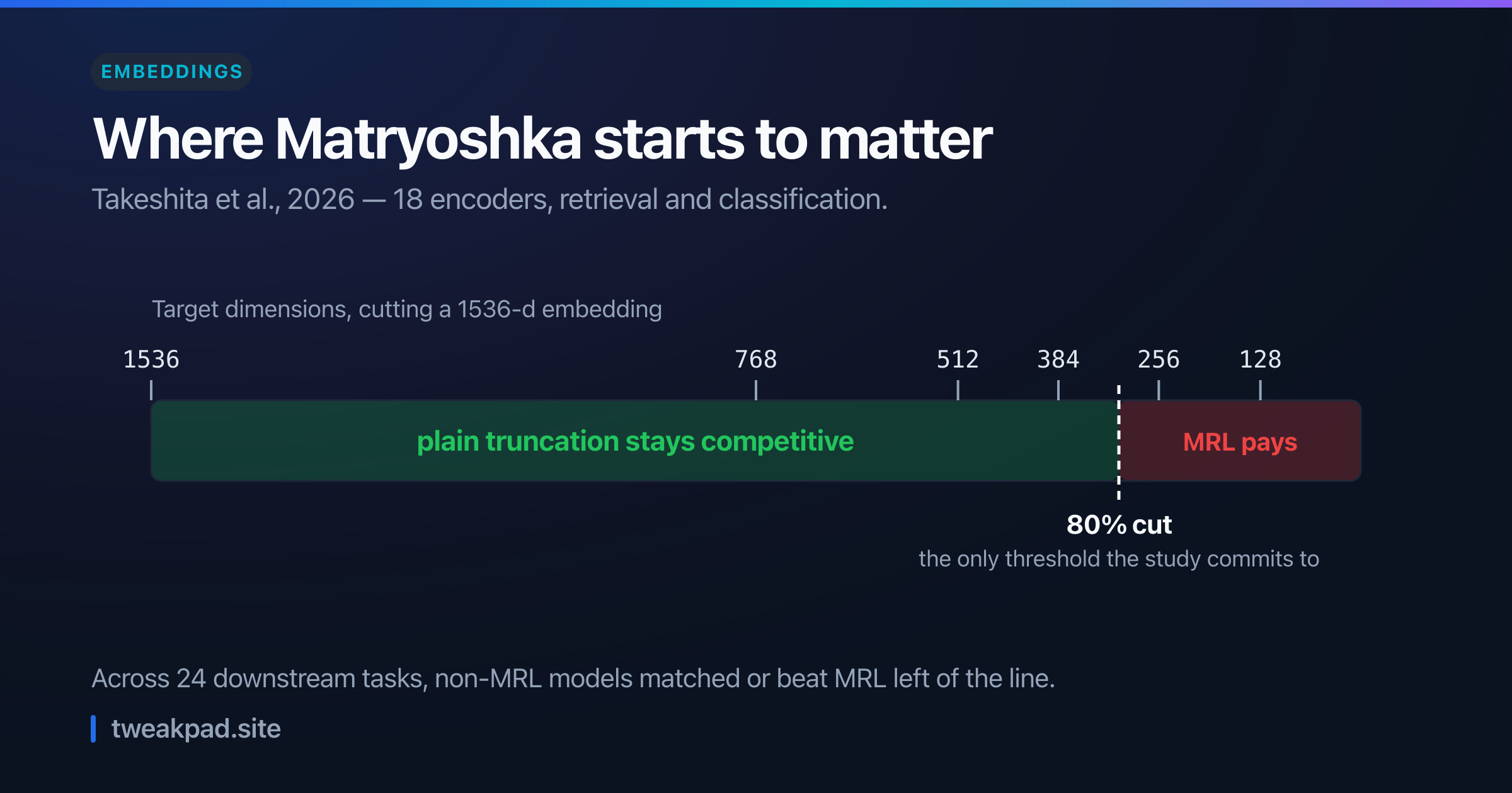
Table of contents
- Key takeaways
- What does truncating embeddings actually cost?
- What Matryoshka training actually does
- The result that inverts the advice
- A worked example
- Truncation or quantization?
- A table for the decision
- Why a prefix works at all is unsettled
- The failure mode, and how to detect it
- What Matryoshka genuinely gets right
- Where this advice is wrong
- The short version
The standard advice on truncating embeddings is that you need a model trained for it. Cut a normal embedding vector short, the story goes, and you destroy it. Only Matryoshka models survive the scissors.
A 2026 study tested that directly across 18 encoders and 24 downstream tasks. Plain truncation held up fine, and often beat the Matryoshka models, right up until you cut about 80%.
Key takeaways#
- Below an 80% cut, ordinary embeddings truncate about as well as Matryoshka ones.
- Earlier work had already put the safe line at 70%, and this study pushed it further.
- Matryoshka training earns its cost in one place: heavy truncation.
- Truncation is a suffix drop, so you never re-embed the corpus.
- If your index uses inner product on unit vectors, re-normalise after cutting.
What does truncating embeddings actually cost?#
Less than you would guess. Truncation drops the trailing elements of each vector, so a 1536-dimension embedding cut to 512 keeps the first 512 numbers and discards the rest. Memory and distance cost fall in proportion, and across 24 tasks the accuracy loss stayed small until the cut got severe.
The cost that does exist is real, though. You lose information, and the question is only where the loss becomes visible.
What Matryoshka training actually does#
Matryoshka Representation Learning, from Kusupati and colleagues at NeurIPS 2022, changes the training objective rather than the model.
A normal encoder optimises one loss on the full vector. MRL instead computes the loss on several nested prefixes of the same vector and adds them up. So the first 8 dimensions get their own loss, the first 16 get one, and so on.
The ladder is short by design. For ResNet50 they used dimensions 8 through 2048, and for BERT-Base a ladder of 12, 24, 48, 96, 192, 384 and 768. They describe this as "optimizing only for O(log(d)) nesting dimensions instead of O(d)", which is roughly 11 checkpoints for a 2048-dimension vector rather than 2048.
Every prefix is therefore trained to work alone. That is the whole idea, and it is elegant. The results were strong too: MRL reached "up to ∼14× smaller representation size for the same accuracy" on ImageNet classification.
The result that inverts the advice#
Here is where the received wisdom and the evidence part company.
Takeshita and colleagues published "To MRL or not to MRL" in May 2026. They applied the same truncation to models trained with and without MRL, which nobody had directly compared before.
Their finding, verbatim: "unless heavily truncating embeddings (i.e. reducing their size by at least 80%), truncated embeddings of non-MRL models are competitive with, and often outperform models trained with MRL".
Read the second half of that. Not merely survivable — often better. The abstract also notes prior work had found "randomly truncating text embeddings has minimal impact in downstream performance unless vectors are reduced in size by at least 70%".
Their recommendation is equally direct: "the additional cost of training with MRL is only beneficial in scenarios where reducing embedding size by about 80% or more is desirable".
A worked example#
Put real numbers on it. Take 10 million documents embedded at 1536 dimensions in float32.
At full width that index holds 10,000,000 × 1536 × 4 bytes, which is 61.44 GB of raw vectors. Cut to 512 dimensions and the same corpus needs 20.48 GB. You just removed 40.96 GB, a 67% cut, and the study puts that comfortably inside the safe zone.
Push to 256 dimensions and you reach 10.24 GB. That is an 83% cut, which lands past the line where MRL starts to matter.
So the decision is sharper than it looks. Going from 1536 to 512 is a large win you can take on any model you already have. Going from 1536 to 256 is the case worth switching models for.
Distance computation scales the same way, since cosine and dot product both walk every dimension. Three times fewer numbers means roughly three times less arithmetic per comparison, which compounds with the graph traversal work we covered in filtered vector search.
Truncation or quantization?#
Cutting dimensions is only one of the two levers on index size, and the other one is often better. So compare them properly before choosing.
Quantization keeps every dimension and shrinks each number. A float32 vector spends 4 bytes per dimension; int8 spends 1, and a binary vector spends an eighth of a byte. Those ratios are definitional, so the memory maths is exact: 4× and 32× respectively.
Run the same 10 million documents through both levers at 512 dimensions. Float32 needs 20.48 GB, int8 needs 5.12 GB, and binary needs 0.64 GB.
Now stack them. Truncating 1536 to 512 is a 3× cut, and int8 adds 4×, so together they take the original 61.44 GB down to 5.12 GB. That is 12× from two changes, neither of which touches your model.
The two levers fail differently, which is the useful part. Truncation discards whole dimensions, so it removes distinctions the tail encoded. Quantization keeps every dimension and coarsens each one, so it blurs fine distances while preserving the shape of the space.
That difference suggests an order of operations. Quantize first, because it is reversible in your pipeline and the quality effect is easy to measure, then truncate only if you still need room. Binary quantization in particular pairs well with a rescoring pass, since a cheap first stage plus an exact second stage is the same two-stage trick that makes tiny vectors useful at all.
A table for the decision#
Here is how I would choose, with the criteria that change the answer.
| Your situation | Do this | Why |
|---|---|---|
| Cutting to 384 or more of 1536 | Truncate the model you have | Non-MRL matched or beat MRL in this range |
| Cutting to 256 or fewer | Switch to an MRL model | The one regime where the training cost pays |
| Already on an MRL model | Truncate to a ladder size | You paid for it, so use the trained prefixes |
| Corpus too expensive to re-embed | Truncate | Dropping a suffix needs no new forward pass |
| Memory is not your bottleneck | Keep full width | There is no prize for a smaller index |
The last row matters more than it reads. Truncation is a cost-reduction technique, so if cost is not hurting, you are trading accuracy for nothing.
Notice also that only one row calls for a model change. That is the practical shape of this finding.
Why a prefix works at all is unsettled#
Worth saying plainly: the paper reports the effect without explaining it.
The authors put it carefully, writing that their results suggest "truncation robustness may not necessarily come from MRL". That is a statement about where the robustness does not come from. Where it does come from is left open.
So resist the tidy story. It is tempting to assume encoders naturally concentrate information in early dimensions, and that would explain the result neatly, but the study did not test that and I am not going to assert it for them.
Treat the mechanism as unknown and the measurement as usable. You do not need to know why a prefix carries the signal in order to check whether it carries yours, and truncating embeddings is cheap enough to test directly.
The failure mode, and how to detect it#
Truncation fails quietly, which is what makes it worth testing rather than assuming.
Nothing throws. Your index builds, queries return, latency improves, and a slice of results is subtly worse. Average similarity scores shift too, so a threshold tuned at full width silently changes meaning.
Measure recall against the full-width index instead. Freeze a few hundred real queries, record the top 20 document IDs at 1536 dimensions, then re-run them at each candidate width and compute overlap. That overlap is your recall proxy, and it needs no human labels.
Make that concrete. If the full-width top 20 for a query and the truncated top 20 share 18 documents, overlap is 0.9, and averaging that over your query set gives one number per width. Anything above roughly 0.95 is usually indistinguishable to a reader, while 0.8 means one result in five moved.
Sweep rather than spot-check. Test 768, 512, 384 and 256, then plot the curve, because your corpus decides where the knee sits and the published 80% describes their models rather than yours.
Run the sweep again whenever you change embedding model. The safe width for truncating embeddings is a property of the encoder, so a model swap invalidates the number you measured, and nothing in your pipeline will announce that.
One more trap worth naming, and the paper does not address it. The authors simply "remove the last elements of the embeddings". If your index stores unit vectors and uses inner product as a stand-in for cosine, that assumption breaks the moment you truncate, since a prefix of a unit vector is not a unit vector. So re-normalise after cutting, or switch the index to true cosine.
What Matryoshka genuinely gets right#
None of this makes MRL a bad idea, and the heavy-truncation case is more common than it sounds.
At very small widths MRL clearly wins, and small widths are exactly what you want for a first-pass filter. The paper's adaptive retrieval result is the striking one: a 16-dimension shortlist followed by 2048-dimension reranking matched full-width retrieval while being "∼128× more efficient in theory and ∼14× faster in practice".
That two-stage shape is the real payoff, and it mirrors the retrieve-wide-then-rerank pattern from reciprocal rank fusion. A tiny vector is not trying to be accurate on its own. It only has to keep the right document in a candidate list.
MRL also gives you one artefact serving many budgets. Mobile can read 64 dimensions and the server can read 768, from the same stored vector, with no second index.
Where this advice is wrong#
One study is not a law. The 2026 paper is careful and broad, covering retrieval on NanoBEIR and BEIR plus MTEB classification, but it is a single result against a widely held belief. Treat 80% as a hypothesis to check on your data, not a constant to trust.
Task type matters and averages hide it. A number aggregated over 24 tasks can conceal a domain where truncation hurts early. Clustering and deduplication lean on fine distinctions between near-identical vectors, and those are the first things a shorter vector blurs.
I have made MRL sound optional. If you are choosing an embedding model today and MRL costs you nothing extra, take it. The finding is that MRL is not a prerequisite for truncating embeddings, not that it is worthless, and having the option costs you nothing when someone else paid for the training.
The short version#
Truncating embeddings does not require a Matryoshka model until you cut hard. Across 18 encoders and 24 tasks, plain truncation matched or beat MRL until roughly an 80% reduction, and earlier work had already found little impact before 70%. So cutting 1536 to 512 is a 40 GB saving you can take on the model you have, while cutting to 256 is the case that justifies switching. Measure recall overlap against your full-width index before and after, and re-normalise if your index assumes unit vectors.
Sources: Kusupati et al., Matryoshka Representation Learning (arXiv:2205.13147), Takeshita et al., To MRL or not to MRL (arXiv:2605.16608)
Tags
- Embeddings
- Vector Search
- AI
- Retrieval