Binary Quantization Works on Your Embeddings, or It Does Not
Binary quantization keeps recall on contrastive embeddings and fails on others. The outcome belongs to your model, not to the method.
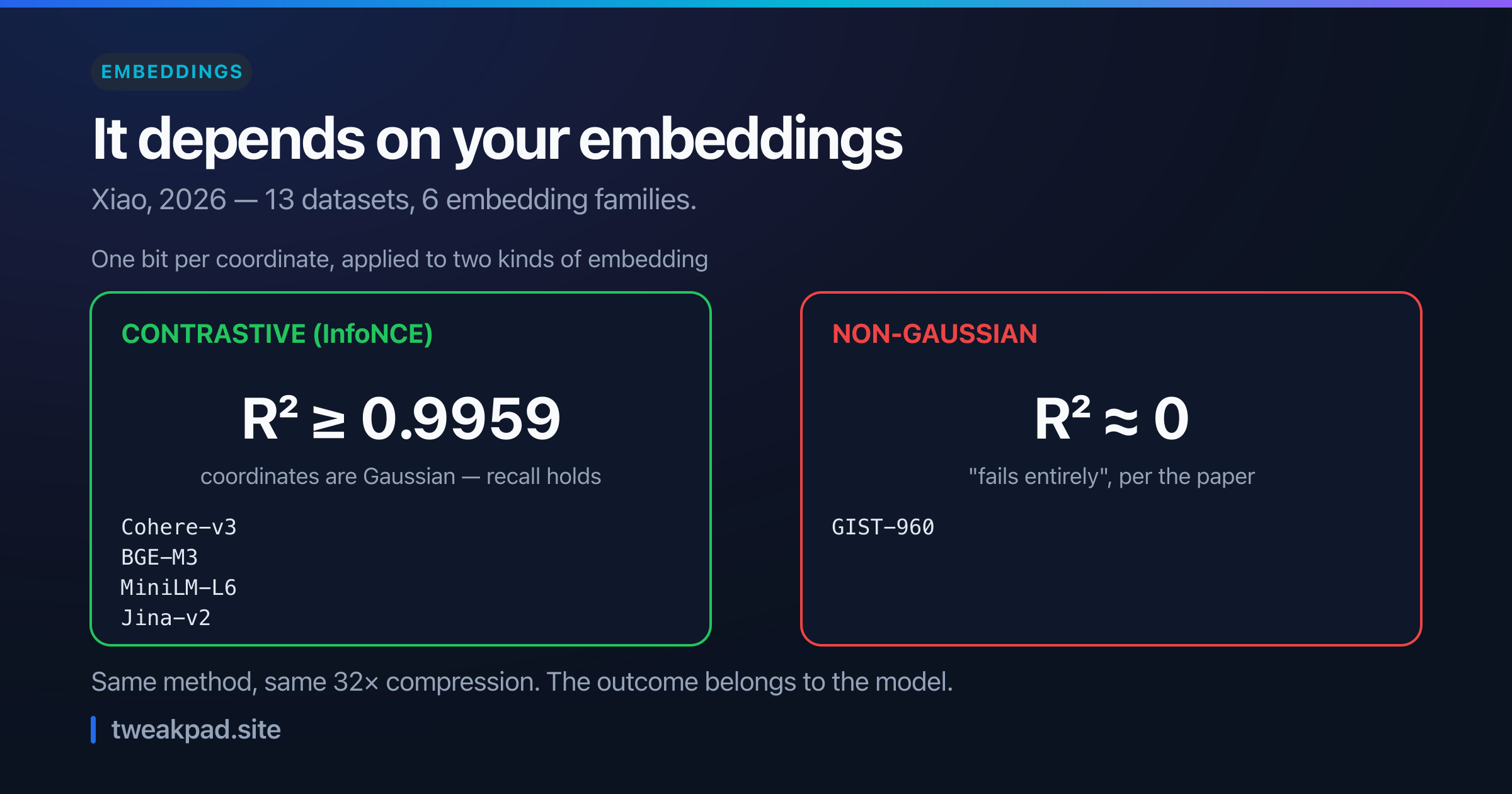
Table of contents
- Key takeaways
- What does binary quantization actually do?
- The claim, and the puzzle underneath
- Why contrastive embeddings survive it
- Coordinate heterogeneity, and why two systems disagree
- A worked example
- A bound instead of a hope
- A table for the decision
- Where the saving actually goes
- The failure mode, and how to detect it
- What rescoring and scalar quantization get right
- Where this advice is wrong
- The short version
The pitch for binary quantization is one number. You get 32× smaller vectors, and you keep most of your recall.
Compression is arithmetic, so that half is always true. Recall is a property of your embedding model, and for some models it does not hold at all.
A 2026 paper puts the puzzle plainly. The technique "achieves competitive recall on contrastive embeddings but fails on others".
Key takeaways#
- The 32× saving is certain. The recall you keep depends on your model.
- Contrastive embeddings survive it, because their coordinates are near-Gaussian.
- One tested non-Gaussian dataset failed the normality check entirely, at R² ≈ 0.
- Two leading systems do opposite things, and copying either blindly can be wrong.
- Adding a second bit bought +0.110 to +0.210 Recall@10 in the same study.
What does binary quantization actually do?#
It throws away everything except the sign. A 1024-dimension float32 vector spends 4 bytes per coordinate. Binary quantization keeps one bit each, recording only whether the value is positive. Distance then becomes a Hamming comparison between bit strings, and that is fast enough to run over the whole index.
The compression is exact and easy to reason about. Whether the surviving bits preserve your rankings is the hard part.
The claim, and the puzzle underneath#
Vendor material tends to present this as a solved trade with a known price. The literature is less settled, and the 2026 paper opens by naming the contradiction.
Yet a striking puzzle persists: BQ achieves competitive recall on contrastive embeddings but fails on others—and two leading systems adopt diametrically opposite strategies (random rotation vs. preserving coordinate axes) without a common theory explaining when each is appropriate.
Two claims worth separating there. The technique works on some embeddings and not others. And the tooling built around it disagrees about the basic approach.
Neither of those is visible in "32× compression, 95% recall".
Why contrastive embeddings survive it#
Most text embedding models train with a contrastive objective. That turns out to matter more than anything about the index.
The paper connects the outcome to the statistical shape of the vectors, reporting a normality check per model family. Contrastive models scored a QQ-plot R² of at least 0.9959, meaning their per-coordinate distributions are almost perfectly Gaussian. The classic GIST-960 image descriptors scored R² ≈ 0 and, in the paper's words, failed entirely.
That is a large gap, and it is not subtle. One family is near-textbook Gaussian and the other is not close.
So the sign bit is a reasonable summary when coordinates are symmetric around zero and similarly scaled. Where they are skewed or wildly uneven, one bit throws away the part that mattered.
Coordinate heterogeneity, and why two systems disagree#
The paper's contribution is naming the variable that decides all this.
The key insight is that coordinate heterogeneity—the non-uniformity of per-coordinate variances—governs the key aspects of BQ performance.
Some dimensions carry more variance than others. That unevenness is itself information, because a Hamming distance over raw coordinates inherits it as an implicit weighting.
Now the practical consequence, which is the part to take away.
random rotation destroys precisely the signal that one paradigm exploits while creating the isotropy that the other requires
Rotation is not a neutral preprocessing step. One family of systems rotates first, because their correction maths assumes isotropy. Another preserves the axes, because the unevenness is what they are exploiting.
Copy a configuration from a system built on the opposite assumption and you remove the thing your approach depended on.
A worked example#
Put real numbers on the compression, since that half is certain.
Take 10 million vectors at 1024 dimensions in float32. That is 10,000,000 × 1024 × 4 bytes, or 40.96 GB of raw vectors. One bit per coordinate takes the same corpus to 1024 bits, so 1.28 GB. The 32× is real.
Now the part that is not free. The same study measured what a second bit buys. Adding a magnitude bit gained +0.110 to +0.210 Recall@10.
So price the alternative. Two bits per coordinate costs 2.56 GB. That is still a 16× saving, and it wins back recall that one bit threw away. Against a 39 GB reduction, the extra 1.28 GB is nothing.
That reframes the decision. The question is rarely whether to compress. It is how many bits to keep, and one bit is an aggressive default to inherit from a blog post.
A bound instead of a hope#
The rigorous treatment of this problem is older, and it exists because ad-hoc quantization was already known to break.
RaBitQ, from SIGMOD 2024, opens with exactly that observation about the prevailing methods.
we note that these methods do not have a theoretical error bound and are observed to fail disastrously on some real-world datasets
Their answer comes with a proof attached. It turns D-dimensional vectors into D-bit strings while guaranteeing "a sharp theoretical error bound". The method rotates to isotropy first, then corrects distances with per-vector scalars.
Notice that RaBitQ is the rotating family from the puzzle above. Its rotation is not a detail. It is what makes the error bound hold, and it is also what erases coordinate heterogeneity.
Two defensible designs, then, resting on incompatible assumptions. That is worth knowing before you mix them.
A table for the decision#
Here is how I would choose, and the first row is the one most people can skip straight to.
| Your situation | Do this | Why |
|---|---|---|
| Modern text embeddings, contrastive | Binary, with rescoring | Coordinates are near-Gaussian |
| Provenance unknown | Run the normality check first | It answers the question in minutes |
| Known non-Gaussian features | Scalar quantization, not binary | Binary failed entirely on that family |
| Recall matters more than RAM | Two bits, not one | Worth up to +0.21 Recall@10 |
| Using a rotating implementation | Do not also hand-tune axes | Rotation already removed that signal |
Row two is cheap insurance. Check the distribution of your own vectors before you commit to an index format. That check costs far less than a re-index.
Row four is where I would push hardest. Teams accept one bit because that is what the marketing said, then spend weeks recovering recall elsewhere.
Where the saving actually goes#
Rescoring is the safety net, and it has a catch I glossed over. The catch decides whether you save anything at all.
To rescore, you need the full-precision vector. So those 40.96 GB still exist somewhere. If you keep them in RAM to make rescoring fast, you did not save memory. You just added an index.
The saving is real when the full vectors live on disk. The binary index stays in RAM and answers the search. Then you read a few hundred full vectors from disk and score those. Few reads, cheap reads.
So the win is not "32× less memory". It is "a hot index in RAM and a cold store on disk", and the ratio depends on how many vectors you touch per query.
Size the oversampling from there. Fetch some multiple of k from the binary index, then rescore that shortlist. Start at 4× and measure overlap against your uncompressed results.
Raise it until the overlap stops improving. That plateau is your number. Most setups find it early, and past it you are paying for disk reads that change nothing.
Watch the disk reads, not just the RAM. An oversample of 20× on a slow volume can cost more latency than the binary index saved, and that trade is easy to miss when you only measure the index.
The failure mode, and how to detect it#
The failure is a quiet quality regression, not an outage. Your index builds and queries return. Latency improves sharply, and a slice of results gets worse in a way no dashboard shows.
Fortunately the paper hands you a diagnostic that runs before you commit. Sample your vectors, take the per-coordinate distributions, and check them against a normal distribution with a QQ plot. Read the R².
Interpret it against their measured range. Near 0.99 puts you with the contrastive models where binary quantization held up. Near zero puts you with the family that failed, and no amount of index tuning fixes the input.
Then measure recall directly rather than trusting the check alone. Freeze a few hundred real queries, record the top 20 IDs from the uncompressed index, and compute overlap against the quantized one. That overlap is your recall proxy and it needs no labels, the same method that works for truncating embeddings.
Re-run both whenever you change embedding model. The statistical shape belongs to the model, so a model swap invalidates the measurement, and nothing in your pipeline will announce that.
What rescoring and scalar quantization get right#
Two things deserve credit before I recommend anything.
Scalar quantization, at 8 bits per coordinate, is the boring option that mostly just works. It keeps every dimension and coarsens each one, so it degrades gracefully rather than falling off a cliff, and it does not care much about your coordinate distributions. A 4× saving that always works beats a 32× saving that sometimes does not.
Rescoring is the other half of the answer, and it is what makes aggressive compression safe. Retrieve a generous candidate list using the compressed vectors, then re-rank those candidates with full-precision distances. The compressed index only has to get the right document into the shortlist.
That is the same two-stage shape as reranking in retrieval, and it works for the same reason. A cheap, slightly wrong first pass is fine when an exact second pass follows it.
Where this advice is wrong#
The scary case may not be yours. GIST-960 is a classic image descriptor set, not a modern embedding model. If you use any mainstream text embedding model, you are almost certainly in the contrastive family that works, and the failure mode is a reason to check rather than a reason to worry.
One paper is not a field. The coordinate-heterogeneity result is recent, covering 13 datasets and 6 embedding families, and it is a theory paper with experiments rather than a decade of practice. Treat the R² check as a useful screen, not as a certified threshold.
Rescoring weakens my own argument. With a good rescoring stage, even a mediocre binary index often recovers acceptable recall, because it only needs the right answer in the candidate set. If you already rescore, the distribution question matters less than I have made it sound, and measuring end-to-end recall is the only test that counts.
The short version#
Binary quantization always gives you the 32× saving and does not always give you the recall. A 2026 analysis found it holds on contrastive embeddings, whose coordinates are near-Gaussian at R² above 0.9959, and fails on a non-Gaussian family that scored close to zero. The governing variable is coordinate heterogeneity, which also explains why one system rotates vectors and another deliberately does not. So check the distribution of your own vectors first, consider two bits rather than one since the second bought up to +0.21 Recall@10, add a full-precision rescoring pass, and measure overlap against your uncompressed index before you trust any of it.
Sources: Xiao, Coordinate Heterogeneity Governs Binary Quantization: From InfoNCE to Recall (arXiv:2605.17524), Gao and Long, RaBitQ: Quantizing High-Dimensional Vectors with a Theoretical Error Bound (arXiv:2405.12497)
Tags
- Embeddings
- Vector Search
- Quantization
- AI